
Fast Accumulation on Streams (2018)

Preface (2023)
Beyond being an interesting solution to a general problem, this algorithm is more relevant than ever given that it describes a scalable solution to creating decentralized provers, an otherwise unsolved issue that plagues zk-rollup implementations today.
My post on the official Mina blog has format-bitrotted over the last five years, barely surviving four blog engine migrations after its original publishing, so I am reposting it here.
Original Post (2018)
While developing Mina, we came across an interesting problem that uncovered a much more general and potentially widely applicable problem: Taking advantage of parallelism when combining a large amount of data streaming in over time. We were able to come up with a solution that scales up to any throughput optimally while simultaneously minimizing latency and space usage. We’re sharing our results with the hope that others dealing with manipulation of online data streams will find them interesting and applicable.
Background
The Mina cryptocurrency protocol is unique in that it uses a succinct blockchain. In Mina the blockchain is replaced by a tiny constant-sized cryptographic proof. This means that in the Mina protocol a user can sync with full-security instantly — users don’t have to wait to download thousands and thousands of blocks to verify the state of the network.
What is this tiny cryptographic proof? It’s called a zk-SNARK, or zero knowledge Succinct Non-interactive ARgument of Knowledge. zk-SNARKs let a program create a proof of a computation, then share that proof with anyone. Anyone with the proof can verify the computation very quickly, in just milliseconds, independent of how long the computation itself takes. While validating proofs is fast, creating them is quite slow, so creating this SNARK proof is much more computationally expensive. We use a few different SNARK proofs throughout Mina’s protocol, but the important one for this post is what we call the "Ledger Proof".
A ledger proof tells us that given some starting account state there was a series of transactions that eventually put us into account state . Let’s refer to such a proof as . So what does it mean for a single transaction to be valid? A transaction, , is valid if it’s been signed by the sender, and the sender had sufficient balance in their account. As a result our account state transitions to some new state . This state transition can be represented as . We could recompute every time there is a new transaction, but that would be slow, with the cost of generating the proof growing with the number of transactions—instead we can reuse the previous proof recursively. These ledger proofs enable users of Mina to be sure that the ledger has been computed correctly and play a part in consensus state verification.
More precisely, the recursive bit of our ledger proof, , or the account state, has transitioned from the starting state to the current state after correct transactions are applied, could naively be defined in the following way:
There exists a proof, , and such that verifies and is valid.
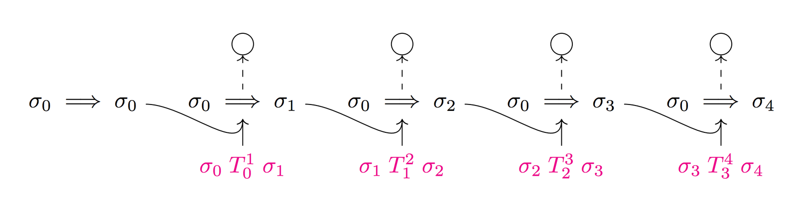
Let’s examine what running this process over four steps would look like:
The functional programming enthusiast will notice that this operation is like a scan:
(* scan [1;2;3] ~init:0 ~f:(fun b a -> b + a) => [1,3,6] *)val scan : 'a list -> ~init:'b -> ~f:('b -> 'a -> 'b) -> 'b list
A scan combines elements of a collection together incrementally and returns all intermediate values. For example if our elements are numbers and our operation is plus, scan [1;2;3] ~init:0 ~f:(fun b a → b + a) has following evaluation trace:
scan [1;2;3] ~init:0 ~f:add(0+1)::(scan [2;3] ~init:(0+1) ~f:add)1::(scan [2;3] ~init:1 ~f:add)1::(1+2)::(scan [3] ~init:(1+2) ~f:add)1::3::(scan [3] ~init:3 ~f:add)1::3::(3+3)::(scan [] ~init:(3+3) ~f:add)1::3::6::(scan [] ~init:6 ~f:add)1::3::6::[][1;3;6]
However, what we really have is a scan operation over some sort of stream of incoming information, not a list. A signature in OCaml may look like this:
val scan : 'a Stream.t -> ~init:'b -> ~f:('b -> 'a -> 'b) -> 'b Stream.t
As new information flows into the stream we combine it with the last piece of computed information and emit that result onto a new stream. Here’s a trace with transactions and proofs:
Unfortunately, we have a serial dependency of proof construction here: you must have before getting . This is very slow. When using Libsnark it takes ~20 seconds to do one of these steps on an 8 core cloud instance, and that’s just for a single transaction. This translates to merely 3 transactions per minute globally on the network!
What we’ll do in this blog post is find a better scan. A scan that maximizes throughput, doesn’t incur too much latency, and doesn’t require too much intermediate state. A scan that takes advantage of properties of the zk-SNARK primitives we have. We’ll do this by iterating on our design until we get something that best meets our requirements. Finally, we’ll talk about a few other potential use cases for such a scan outside of cryptocurrency.
Requirements
Now that we understand the root problem, let’s talk about requirements to help guide us toward the best solution for this problem. We want to optimize our scan for the following features:
-
Maximize transaction throughput: Transaction throughput here refers to the rate at which transactions can be processed and validated in the Mina protocol network. Mina strives to be able to support low transaction fees and more simultaneous users on the network, so this is our highest priority.
-
Minimize transaction latency: It’s important to minimize transaction latency to enter our SNARK to keep the low RAM requirements on proposer nodes, nodes that propose new transitions during Proof of Stake. SNARKing a transaction is not the same as knowing a transaction has been processed, so this is certainly less important for us than throughput.
-
Minimize size of state: Again, to keep low RAM requirements on proposer nodes we want to minimize the amount of data we need to represent one state.
And moreover, this is the order of importance of these goals from most to least important: Maximize throughput, minimize latency, minimize size of state.
Properties
We’ll start with some assumptions:
- All SNARK proofs take one unit of time to complete
- Transactions arrive into the system at a constant rate per unit time
- We effectively have any number of cores we need to process transactions because we can economically incentivize actors to perform SNARK proofs and use transaction fees to pay those actors.
- Two proofs can be recursively merged:
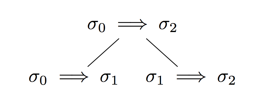
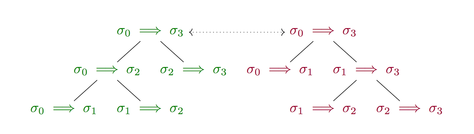
This merge operation is associative:
So we can actually write transaction SNARKs that effectively prove the following statements:
Base ()
There exists such that the transaction is valid
Merge ()
There exists and such that both proofs verify
Before we go any further, though, let's abstract away some details here.
Abstractions
Data:
Base work:
Merge work:
Accumulated value:
Let’s say that data effectively enqueues a "Base job" that can be completed to become "Base work". Similarly, two "Base work"s (or two "Merge works"s) can be combined in a "Merge job” to create "Merge work".
Initial Analysis
Upper Bound
Let’s set an upper bound efficiency target for any sort of scan. No matter what we do we can’t do better than the following:
- Throughput: per unit time
We said new data was entering the system at a rate of per unit time, so the best we can do is complete the work as soon as it’s added.
- Latency:
In the best case, we don’t have to wait to get the piece of data included as part of the scan result. Whatever time it takes to do one step is the time it takes before our data is included in the scan result.
- Space:
We don’t need to store any extra information besides the most recent result.
As a reminder, we decided that the naive approach is just a standard linear scan. This “dumb scan” can be a nice lower bound on throughput, we can also analyze the other attributes we care about here:
Linear Scan
- Throughput: per unit time
Our linear scan operation emits a result at every step and so we need the prior result before we can perform the next step.
- Latency:
Every step emits a single result based on the data
- Space:
We only have to hold on to the most recently accumulated result to combine with the next value.
Since our primary goal is to maximize throughput, it’s clear a linear scan isn’t appropriate.
Parallel Periodic Scan
Recall that the merge operation is associative. This means that we can choose to evaluate more than one merge at the same time, thus giving us parallelism! Even though data are coming in only at a time, we can choose to hold more back to unlock parallel merge work later. Because we effectively have infinite cores we can get a massive speedup by doing work in parallel.
This gives rise to the notion of a “periodic scan”:
(* periodicScan 1->2->3->4->5->6->7->8 ~init:0 ~lift:(fun a -> a) ~merge:(fun a b -> a + b) => 10->36*)val periodicScan : 'a Stream.t -> ~init:'b -> ~lift:('a -> 'b) -> ~merge:('b -> 'b -> 'b) -> 'b Stream.t
A scan that periodically emits complete values, not every time an 'a datum appears on a stream, but maybe every few times. This therefore has slightly different semantics than a traditional scan operation.
Rather than returning a stream emitting 1→3→6→10→15→21→28→36, we buffer data elements 1 through 4 and compute with those in parallel, and only emit the resulting sum, 10, when we’re done. Likewise we buffer 5 through 8, and combine that with 10 and emit that 36 when we’re done. We periodically emit intermediate results instead of doing so every time.
Naive Implementation of Periodic Scan
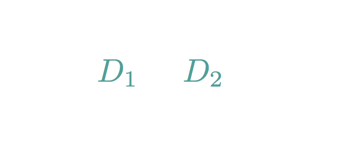
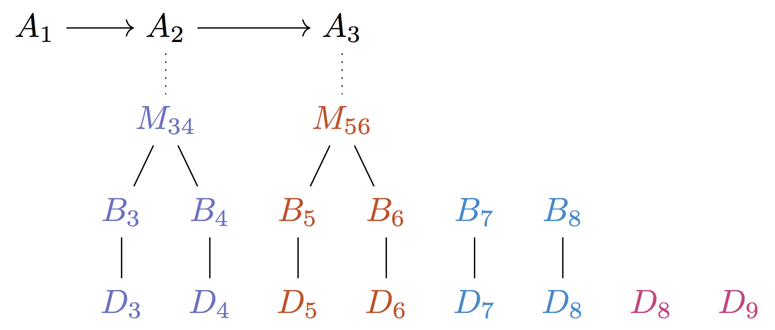
Let's go over this tree construction step-by-step, considering what happens to our data over time as it’s coming through into the system. Let’s consider .
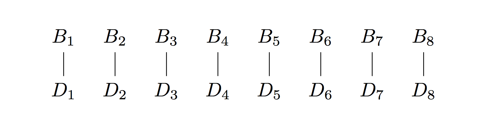
First we gather pieces of data and enqueue Base jobs for our network to complete. We use of our cores and can complete all jobs in one time step. We hold back the data on the pipe, and we are forced to buffer it because we haven’t finished handling the first .
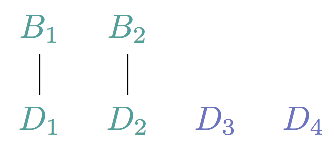
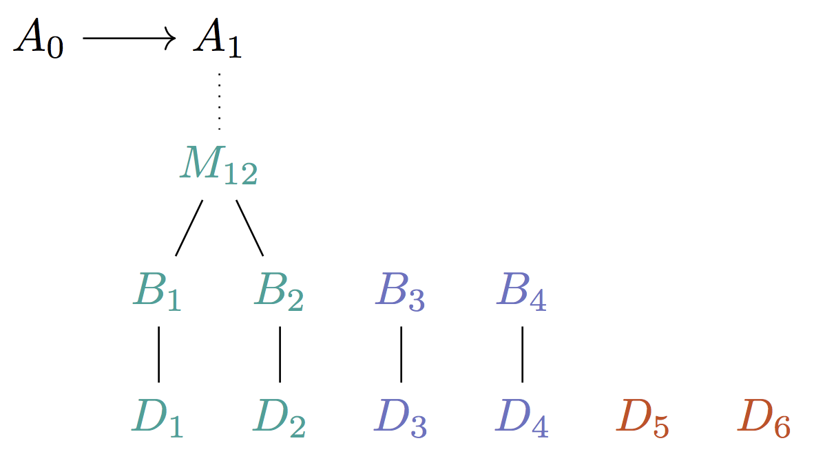
As we add Base work, we give way for a series of Merge jobs that can be completed in the next step:
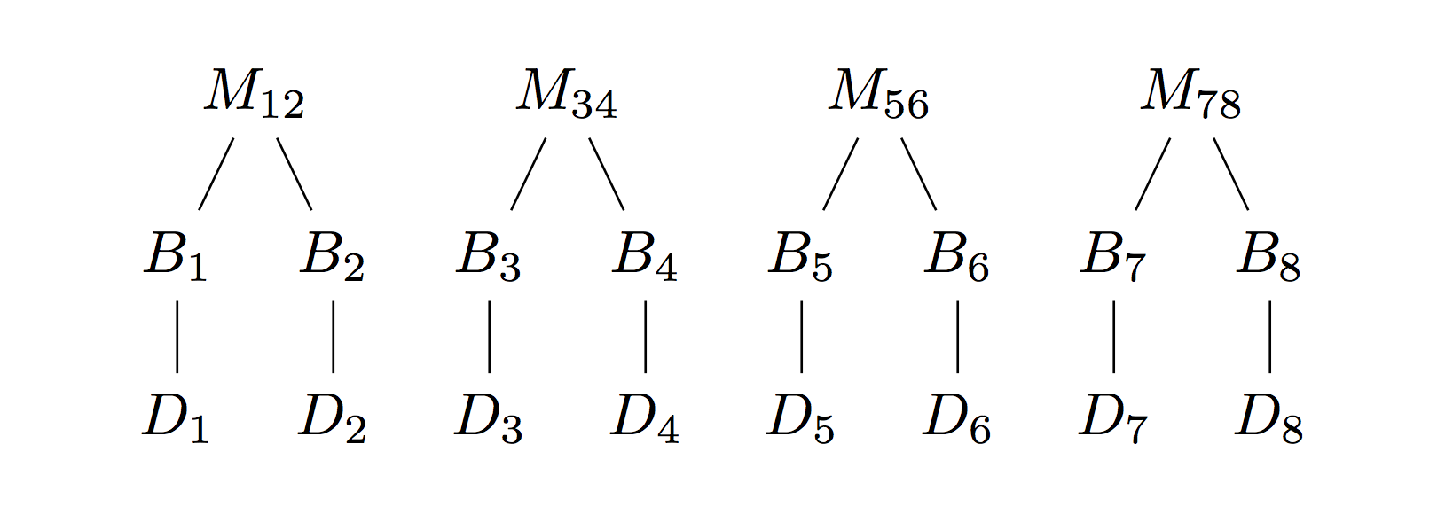
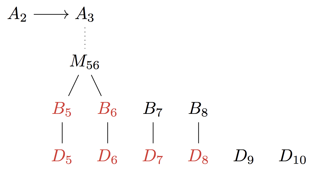
Now we have pieces of merge work to complete and we use cores and complete them in one time step.
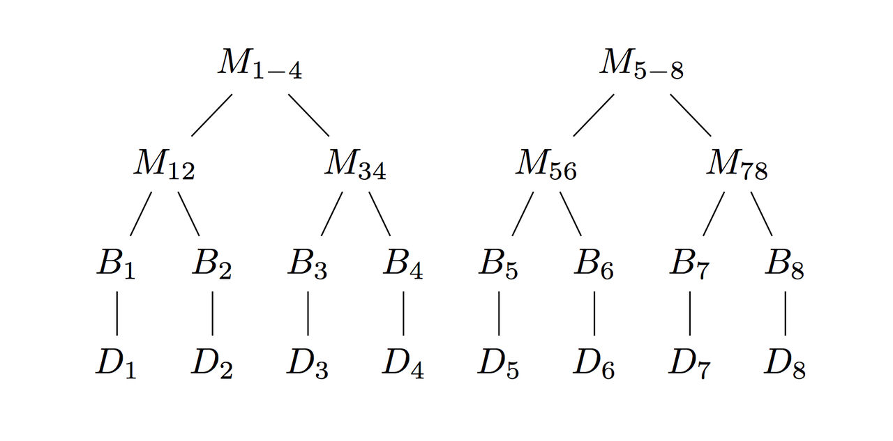
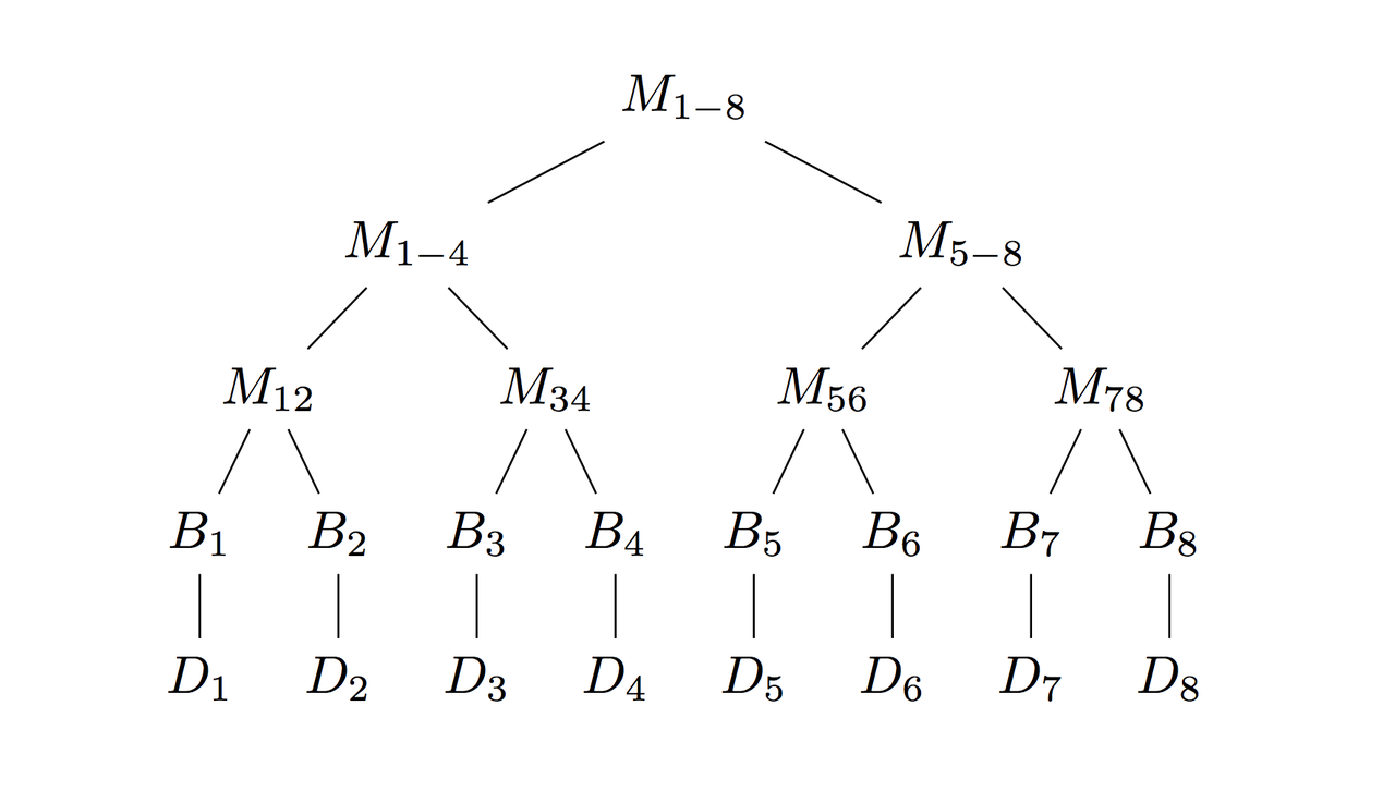
We repeat until we reach the top of the tree. The completed Merge work at the top can be consumed by the rest of the system.
Analysis
- Throughput:
Every steps, we have the opportunity to consume more pieces of data.
- Latency:
It takes time steps before we emit our top-level merge work as we half the nodes in each layer of our tree at each step.
- Space:
We now have to keep parts of a tree around at each step. Since our trees have leaves, typical binary trees have nodes when completed, and we have an extra layer, we actually use nodes.
Naive Periodic Scan
For the purposes of visualization, unit time is being replaced with 60 seconds. We assume the space of a single node in the tree is 2KB.
| Throughput (in data per second) | Latency (in seconds) | Space (in bytes) | |
|---|---|---|---|
| 0.0333 | 180 | ~22KB | |
| 0.0667 | 300 | ~94KB | |
| 1.71 | 660 | ~6MB | |
| 19.5 | 900 | ~98MB |
Serial Scan
| Throughput (in data per second) | Latency (in seconds) | Space (in bytes) | |
|---|---|---|---|
| 0.05 | 20 | ~2KB | |
| 0.05 | 20 | ~2KB | |
| 0.05 | 20 | ~2KB | |
| 0.05 | 20 | ~2KB |
We have increased throughput at the cost of some latency and space when compared with the serial approach, so this is a little bit better!
However, this solution leaves something to be desired—why must we halve our parallelism as we walk up each layer of the tree? We have a stream feeding us data values every unit of time, so we should have enough work to do. Shouldn’t we use this somehow?
Better Solution
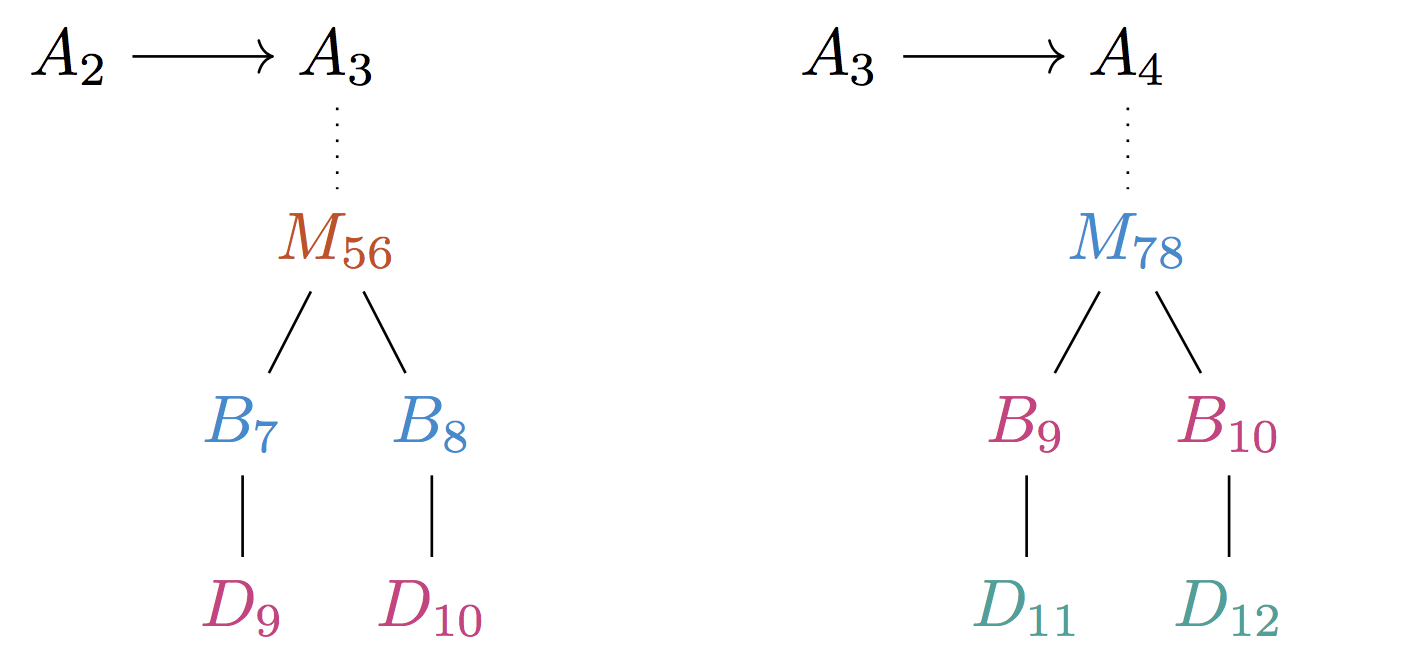
Let's take advantage of the fact that we get new data values each time we complete work—still preferring earlier queued data values to minimize latency once we've exhausted available parallelism.
With this in mind, let's trace a run-through, this time always making sure we have pieces of work to do at every step—for illustration, let's pick :
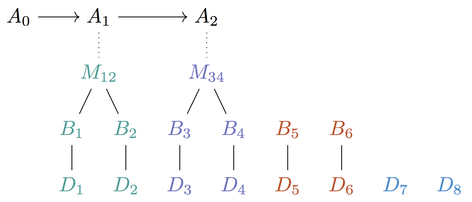
We do as we did before, but this time we have jobs to complete and can dispatch to our cores every step. We have exactly trees pending at a time. At every step, we complete the first tree (tree zero) and at tree , we complete layer .
Analysis
- Throughput:
Throughput of work completion matches our stream of data! It’s perfect, we’ve hit our upper-bound.
- Latency:
Latency is still logarithmic, though now it’s steps as our trees have leaves and we an extra layer on the bottom for base jobs. In fact, this is actually the lower bound.
- Space:
We have multiple trees now. Interestingly, we have exactly trees pending at a time. Again our longer trees take up an extra layer than traditional binary trees, so in this case nodes since we have leaves, and we have of these trees.
Now that we have thoroughly optimized our throughput and latency, let’s optimize for space.
Optimize size
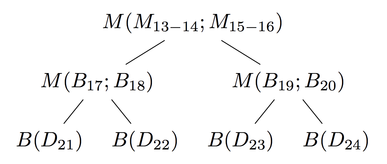
Do we really need to hold all trees? We only ever care about the frontier of work. All the information we need to perform the next layer of jobs. We clearly don’t need to store anything above that or below it in the trees.
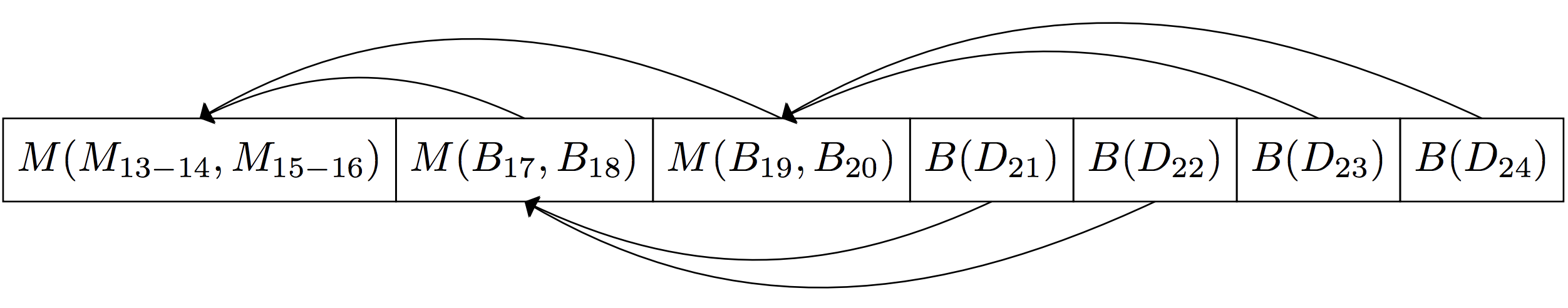
Notice that we only use some of each layer of trees even across the trees. And so we can represent the frontier of the trees with only a single tree representing the work pipeline moving from leaves to the root in the following manner:
Analysis
- Throughput:
Throughput is the same as before.
- Latency:
Latency is the same as above.
- Space:
We’ve reduced our space back down to a single tree with leaves .
Space Optimization
Do we really need that extra layer? If we change how we think about the problem, we can use a perfect binary tree which we can manipulate to save even more space:
Now we’re down to nodes—a standard binary tree with leaves.
How do we store the tree? Since we know the size a priori (a complete binary tree with leaves), we can use a succinct representation.
A succinct data structure requires only extra space to manage the relationship between the elements if is the optimal number of bits that we need to express the information in an unstructured manner. Note that this is little- not big-—a much tighter bound.
In fact our structure as described is actually an implicit one because of our scalar cursor. An implicit data structure is one that uses only extra bits. In later refinements (in part 2), we'll go back to a succinct representation because we need to relax one of the assumptions we made here. This is similar to the popular implicit heap that you may have learned about in a computer science class.
Final Analysis
- Throughput:
Throughput keeps up with production rate , so we couldn’t do better.
- Latency:
Latency is proportional to steps, as we described earlier, so we don’t get hurt too badly there.
- Space:
We have an implicit data structure representation for our complete binary tree with leaves as described above.
Fully Optimized Scan
| Throughput (in data per second) | Latency (in seconds) | Space (in bytes) | |
|---|---|---|---|
| 0.0667 | 180 | ~22KB | |
| 0.267 | 300 | ~94KB | |
| 17.1 | 660 | ~6MB | |
| 273 | 900 | ~98MB | |
| 1092 | 1020 | ~393MB |
We went from a sequential solution that at only handled a throughput of 0.05 data per second to an initial parallel solution that handled 19.5 data per second to a fully optimized solution that handles 273 data per second. Our final solution even has optimal latency and space characteristics.
We did it! Mina can now be limited in its throughput by the speed at which information can flow across the network, and no longer by the time it takes to construct a SNARK. Moreover, we solved a more general problem: Efficiently computing an online periodic parallel scan over an infinite stream for some associative operation.
Other Use Cases
Deep space telescopes produce an astronomical amount of data per second. For example, the Square Kilometre Array will process petabits of data per second. If data frames are coming in faster than we can process them which is certainly true for some types of workloads like non-parametric machine learning, we can use this data structure to handle these streams.
More generally, certain map-reduce type workloads that act in an online fashion (on an infinite stream of inputs instead of a finite collection) with expensive operators, could benefit from using our same data structure.
You can also go through literature and try to find prior art. We didn’t find much searching through map-reduce papers. The only thing that was a bit related is a paper from the GPU programming world, but doesn’t address the infinite streaming bit. Please tweet @bkase_ if you want to share any related work.
Conclusion
We were able to take advantage of parallelism and other properties of our system to materialize this general “periodic scan” problem of combining data streaming in online fashion which as we described doesn’t limit throughput at all, has optimal latency characteristics, and is succinct. With this data structure, Mina is free to take advantage of succinctness to offer a high-throughput with no risk of centralization!
Future work
We’ll explore modifying this structure to optimize latency in the presence of variable throughput. You can imagine that relaxing constraints on whether scan tree nodes need to be filled with genuine proofs or "empty dummies" can help here.
Additionally, we will want to explore a more efficient mechanism to share account states that are part of the scan tree to nodes that don’t care about the in-progress proofs, so that bandwidth-constrained nodes can still look up their most recent account states without waiting for a ledger proof to pop out of the tree.
Appendix
We can reify this model with the following signature in the Mina codebase:
val start : parallelism_log_2:int -> ('a, 'd) State.t(** The initial state of the parallel scan at some parallelism *)val next_jobs : state:('a, 'd) State.t -> ('a, 'd) Available_job.t list(** Get all the available jobs *)val enqueue_data : state:('a, 'd) State.t -> data:'d list -> unit Or_error.t(** Add data to parallel scan state *)val free_space : state:('a, 'd) State.t -> int(** Compute how much data ['d] elements we are allowed to add to the state *)val fill_in_completed_jobs : state:('a, 'd) State.t -> completed_jobs:'a State.Completed_job.t list -> 'a option Or_error.t(** Complete jobs needed at this state -- optionally emits the ['a] at the topof the tree *)
Acknowledgements
Thanks to Evan Shapiro for working through these data structures with me when we were first figuring this stuff out. Thanks to Deepthi Kumar for collaborating with me on several optimizations. Thanks to Laxman Dhulipala for taking a video call early on and helping with an early core insight about the multiple trees. Finally, thanks to Omer Zach and Ember Arlynx (and Evan and Deepthi) for their very thorough feedback on drafts of this post!